Matrix for linear systems

I used to wonder, "What the hell are people doing with these rectangle arrays just to solve linear equations?" Back when I was a kid, teachers just taught the how and never the why. It felt like extra work for no reason.

It wasn't until my degree and now my Master’s that it finally clicked. My brain processes these things much better when there’s a reason behind the madness. If you’ve ever felt like matrices were just a boring way to rewrite math, this is for you.

The "What" and "Why"

Simply put, a matrix is a rectangular array of numbers arranged in rows and columns.

But that’s just the definition. The real question is: why do we use matrices?

Matrices are a structured way to store numbers. They help represent information in a clean, organized format. Instead of dealing with messy equations full of variables, we can focus purely on numbers in a systematic way.

For example, instead of writing:

x + y + z = 3
2x - y + z = 5

We can rewrite this in a compact form:

Ax = b

I’ll explain this form in a bit.

Another important reason: computers are not like us. They don’t “understand” equations the way we do. They need structured data. Matrices provide exactly that a consistent and efficient way to represent and process systems of equations.

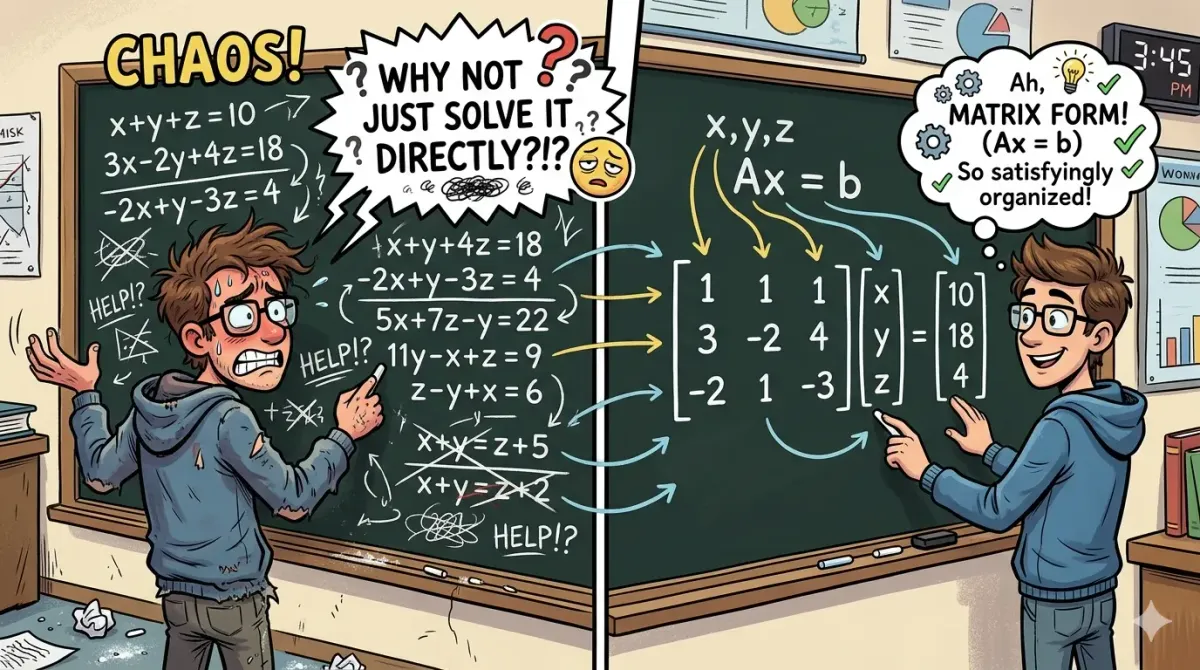
From Chaos to Ax = b

Consider a system like this:

a1x + b1y + c1z = d1
a2x + b2y + c2z = d2
a3x + b3y + c3z = d3

We can represent this using matrices as:

Ax = b

Where:

• A = coefficient matrix
• x = variable matrix (column vector)
• b = right-hand side (RHS) column vector

So it becomes:

[ a1 b1 c1 ] [ x ] [ d1 ]
[ a2 b2 c2] [ y ] = [ d2 ]
[ a3 b3 c3] [ z ] [ d3 ]

Now instead of dealing with multiple equations, we deal with one compact matrix equation.

To solve this system, we use Gaussian Elimination.

This method has three main steps:

Step 1: Form the Augmented Matrix

We combine matrix A and vector b into one matrix:

[ a1 b1 c1 | d1 ]
[ a2 b2 c2 | d2 ]
[ a3 b3 c3 | d3 ]

This is called the augmented matrix (A | b).

Step 2: Row Operations → Upper Triangular Form

We transform the matrix into an upper triangular form using row operations.

An upper triangular matrix looks like this:

[ * * * ]
[ 0 * * ]
[ 0 0 * ]

(Everything below the diagonal becomes zero.)

The result becomes:

(U | b′)

Where:

• U is the upper triangular matrix
• b′ is the updated RHS vector

Step 3: Back Substitution

Now we solve from bottom to top:

• First solve for the last variable
• Then substitute upwards

This is called back substitution.

Allowed Elementary Row Operations

To move from step 1 to step 2, we use these operations:

1. Swap two rows
2. Multiply a row by a non-zero constant
3. Add a multiple of one row to another row

These operations do not change the solution—they just simplify the system.

Example

Let’s go through a simple example:

x + y + z = 6
2x + 3y + z = 10
x + 2y + 3z = 13

Step 1: Augmented Matrix

[ 1 1 1 | 6 ]
[ 2 3 1 | 10 ]
[ 1 2 3 | 13 ]

Step 2: Row Operations

Make zeros below the first pivot:

• R2 → R2 - 2R1
• R3 → R3 - R1

[ 1 1 1 | 6 ]
[ 0 1 -1 | -2 ]
[ 0 1 2 | 7 ]

Now eliminate below second pivot:

• R3 → R3 - R2

[ 1 1 1 | 6 ]
[ 0 1 -1 | -2 ]
[ 0 0 3 | 9 ]

Step 3: Back Substitution

From last row:

3z = 9 → z = 3

Second row:

y - z = -2 → y - 3 = -2 → y = 1

First row:

x + y + z = 6 → x + 1 + 3 = 6 → x = 2

Final Answer:

x = 2
y = 1
z = 3

Final Thoughts

I still have a lot more to add about matrices. we’ve only scratched the surface and there’s a whole lot more to discuss. But that’s for another day, since I need to go through some lecture recordings to better understand data modeling.

Bye for today. Let’s meet next day with something new 🙂